안녕하세요, 데 박입니다.
오늘은 머신러닝을 배운다면 꼭 알아야할 머신러닝 모델,
SVM (Support Vector Machine)에 대해서 공부해보도록 하겠습니다.

□ SVM (Support Vector Machine)
SVM은 매우강력한 선형, 비선형 분류, 회귀 이상치 탐색에도 사용할 수 있는 다목적 머신러닝 모델입니다.
머신러닝에서 인기있는 모델에 속하고 SVM은 특히 복잡한 분류 문제에 잘 들어맞으며 작거나 중간 크기의 데이터셋에 적합합니다. 또한 이 글에서는 선형, 비선형 분류를 다루었으니 이 점 참고해주시길 바라겠습니다.
□ 라지마진분류
from sklearn.svm import SVC
from sklearn import datasets

iris = datasets.load_iris()
X = iris["data"][:, (2, 3)]  # 꽃잎 길이, 꽃잎 너비
y = iris["target"]

setosa_or_versicolor = (y == 0) | (y == 1)
X = X[setosa_or_versicolor]
y = y[setosa_or_versicolor]

# SVM 분류 모델
svm_clf = SVC(kernel="linear", C=float("inf"))
svm_clf.fit(X, y)
plt.style.use('dark_background')
# 나쁜 모델
x0 = np.linspace(0, 5.5, 200)
pred_1 = 5*x0 - 20
pred_2 = x0 - 1.8
pred_3 = 0.1 * x0 + 0.5
def plot_svc_decision_boundary(svm_clf, xmin, xmax):
w = svm_clf.coef_[0]
b = svm_clf.intercept_[0]
# 결정 경계에서 w0*x0 + w1*x1 + b = 0 이므로
# => x1 = -w0/w1 * x0 - b/w1
x0 = np.linspace(xmin, xmax, 200)
decision_boundary = -w[0]/w[1] * x0 - b/w[1]
margin = 1/w[1]
gutter_up = decision_boundary + margin
gutter_down = decision_boundary - margin
svs = svm_clf.support_vectors_
plt.scatter(svs[:, 0], svs[:, 1], s=180, facecolors='#FFAAAA')
plt.plot(x0, decision_boundary, "w-", linewidth=2)
plt.plot(x0, gutter_up, "w--", linewidth=2)
plt.plot(x0, gutter_down, "w--", linewidth=2)
fig, axes = plt.subplots(ncols=2, figsize=(12,5), sharey=True)
plt.sca(axes[0])
plt.plot(x0, pred_1, "g--", linewidth=2)
plt.plot(x0, pred_2, "m-", linewidth=2)
plt.plot(x0, pred_3, "r-", linewidth=2)
plt.plot(X[:, 0][y==1], X[:, 1][y==1], "bs", label="Iris versicolor")
plt.plot(X[:, 0][y==0], X[:, 1][y==0], "yo", label="Iris setosa")
plt.xlabel("Petal length", fontsize=14)
plt.ylabel("Petal width", fontsize=14)
plt.legend(loc="upper left", fontsize=14)
plt.axis([0, 5.5, 0, 2])
plt.sca(axes[1])
plot_svc_decision_boundary(svm_clf, 0, 5.5)
plt.plot(X[:, 0][y==1], X[:, 1][y==1], "bs")
plt.plot(X[:, 0][y==0], X[:, 1][y==0], "yo")
plt.xlabel("Petal length", fontsize=14)
plt.axis([0, 5.5, 0, 2])
plt.show()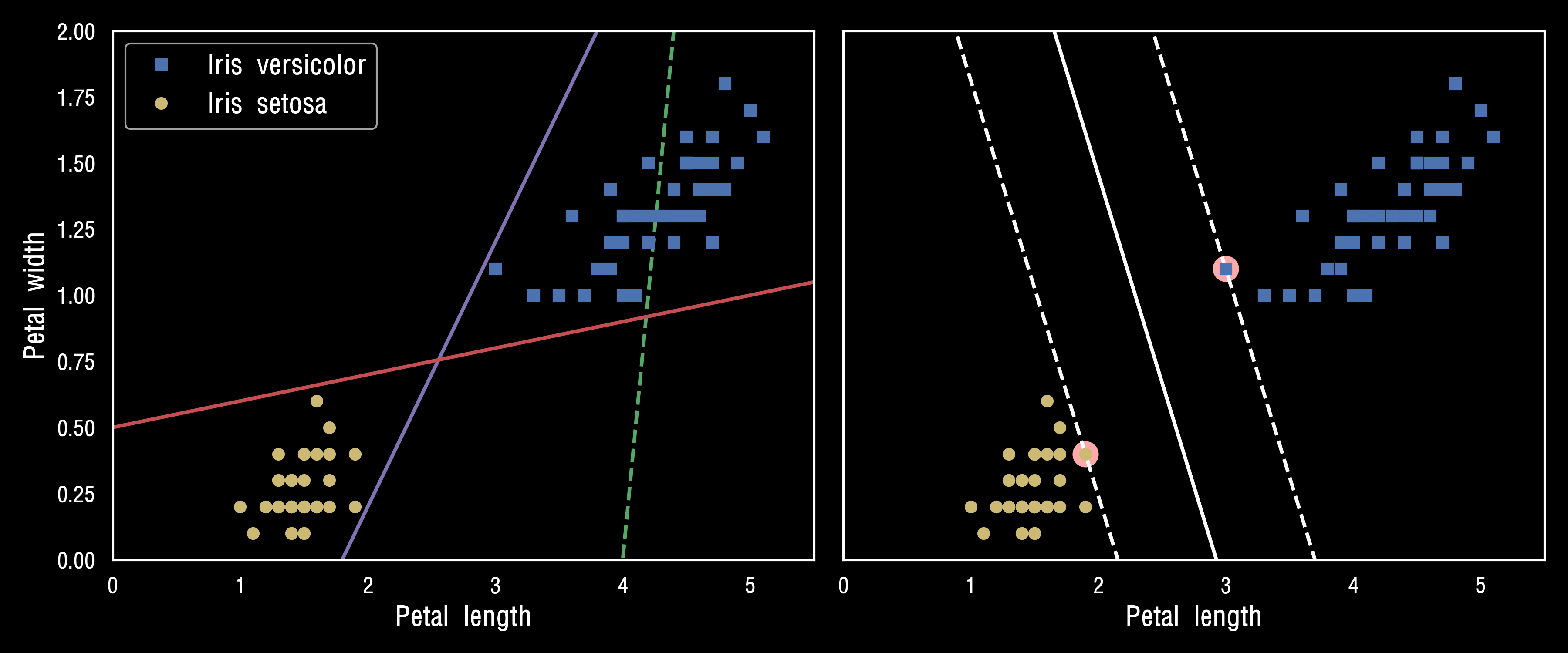
왼쪽 그래프에서 3개의 선형 분류기에서 만들어진 결정경계가 보입니다.
점선으로 나타난 결정 경계를 만든 모델은 클래스를 적절하게 분류하지 못하고 있습니다.
다른 두 모델은 훈련셋에 대해 완벽하게 동작합니다. 하지만 결정경계가 샘플에 너무 가까워 새로운 샘플에 대해서는 아마 잘 작동하지 못할 것입니다.
오른쪽 그래프에 있는 실선은 SVM 분류기의 결정 경계입니다.
이 직선은 두개의 클래스를 나누고 있을 뿐만 아니라 제일 가까운 훈련샘플로부터 가능한 한 멀리 떨어져 있습니다
SVM 분류계를 클래스 사이에 가장 폭이 넓은 도로를 찾는 것으로 생각할 수 있습니다.
그래서 "라지 마진 분류 (Large Margin Classification)"이라고 합니다.
도로 바깥쪽에 훈련 샘플을 더 추가해도 결정 경계에는 전혀 영향을 미치지 않습니다.
도로 경계에 위치한 샘플에 의해 전적으로 결정(또는 지지, support)됩니다.
이런 샘플을 서포트 벡터(support vector)라고 합니다. 그림에 분홍생 동그라미로 표시되었습니다.
Xs = np.array([[1, 50], [5, 20], [3, 80], [5, 60]]).astype(np.float64)
ys = np.array([0, 0, 1, 1])
svm_clf = SVC(kernel="linear", C=100)
svm_clf.fit(Xs, ys)
plt.style.use('dark_background')

plt.figure(figsize=(9,4))
plt.subplot(121)
plt.plot(Xs[:, 0][ys==1], Xs[:, 1][ys==1], "bo")
plt.plot(Xs[:, 0][ys==0], Xs[:, 1][ys==0], "ms")
plot_svc_decision_boundary(svm_clf, 0, 6)
plt.xlabel("$x_0$", fontsize=20)
plt.ylabel("$x_1$", fontsize=20, rotation=0)
plt.title("Unscaled", fontsize=16)
plt.axis([0, 6, 0, 90])

from sklearn.preprocessing import StandardScaler
scaler = StandardScaler()
X_scaled = scaler.fit_transform(Xs)
svm_clf.fit(X_scaled, ys)

plt.subplot(122)
plt.plot(X_scaled[:, 0][ys==1], X_scaled[:, 1][ys==1], "bo")
plt.plot(X_scaled[:, 0][ys==0], X_scaled[:, 1][ys==0], "ms")
plot_svc_decision_boundary(svm_clf, -2, 2)
plt.xlabel("$x'_0$", fontsize=20)
plt.ylabel("$x'_1$  ", fontsize=20, rotation=0)
plt.title("Scaled", fontsize=16)
plt.axis([-2, 2, -2, 2])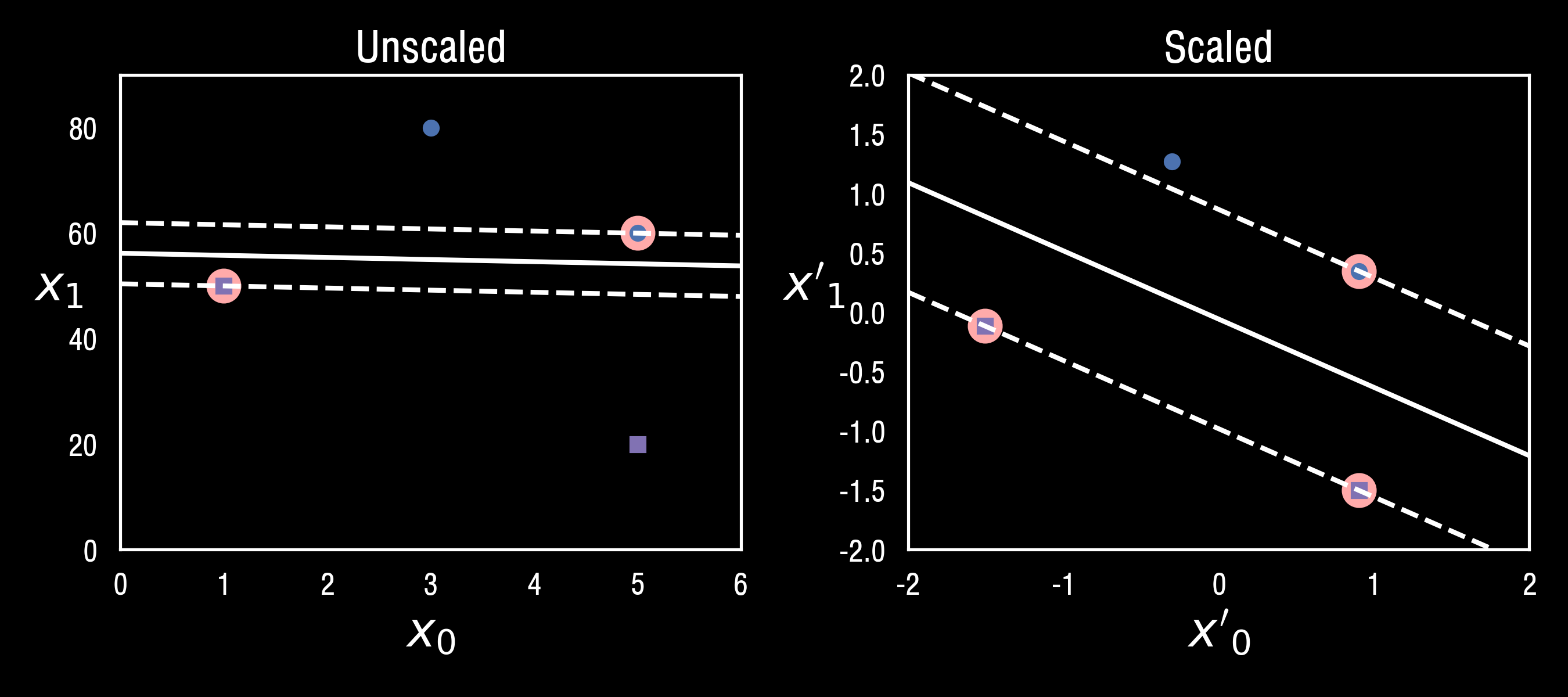
SVM은 특성의 스케일에 민감합니다. 위의 그림의 왼쪽그래프에서 Y축의 스케일이 X축의 스케일보다 훨씬 커서 가장 넓은 도로가 거의 수평에 가깝게 됩니다.
특성의 스케일을 조정하면 결정경계가 훨씬 좋아집니다! (scikit-learn의 preprocessing모듈에서 StandardScaler로 간편하게 표준화시킬 수 있습니다.)
□ 소프트 마진 분류
X_outliers = np.array([[3.4, 1.3], [3.2, 0.8]])
y_outliers = np.array([0, 0])
Xo1 = np.concatenate([X, X_outliers[:1]], axis=0)
yo1 = np.concatenate([y, y_outliers[:1]], axis=0)
Xo2 = np.concatenate([X, X_outliers[1:]], axis=0)
yo2 = np.concatenate([y, y_outliers[1:]], axis=0)

svm_clf2 = SVC(kernel="linear", C=10**9)
svm_clf2.fit(Xo2, yo2)

fig, axes = plt.subplots(ncols=2, figsize=(10,2.7), sharey=True)

plt.sca(axes[0])
plt.plot(Xo1[:, 0][yo1==1], Xo1[:, 1][yo1==1], "bs")
plt.plot(Xo1[:, 0][yo1==0], Xo1[:, 1][yo1==0], "yo")
plt.text(0.3, 1.0, "불가능!", fontsize=24, color="red")
plt.xlabel("Petal length", fontsize=14)
plt.ylabel("Petal width", fontsize=14)
plt.annotate("이상치",
             xy=(X_outliers[0][0], X_outliers[0][1]),
             xytext=(2.5, 1.7),
             ha="center",
             arrowprops=dict(facecolor='black', shrink=0.1),
             fontsize=16,
            )
plt.axis([0, 5.5, 0, 2])

plt.sca(axes[1])
plt.plot(Xo2[:, 0][yo2==1], Xo2[:, 1][yo2==1], "bs")
plt.plot(Xo2[:, 0][yo2==0], Xo2[:, 1][yo2==0], "yo")
plot_svc_decision_boundary(svm_clf2, 0, 5.5)
plt.xlabel("Petal length", fontsize=14)
plt.annotate("이상치",
             xy=(X_outliers[1][0], X_outliers[1][1]),
             xytext=(3.2, 0.08),
             ha="center",
             arrowprops=dict(facecolor='black', shrink=0.1),
             fontsize=16,
            )
plt.axis([0, 5.5, 0, 2])

save_fig("sensitivity_to_outliers_plot")
plt.show()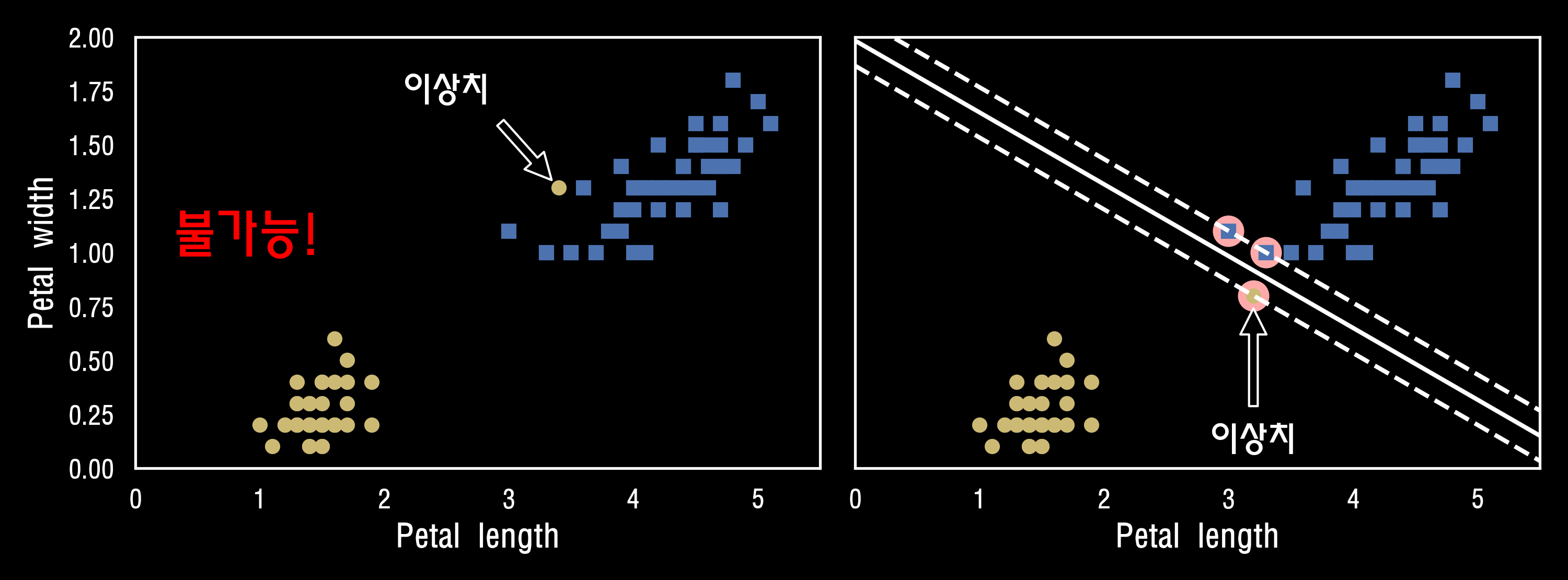
모든 샘플이 도로 바깥쪽에 올바르게 분류되었다면 이를 "하드 마진 분류" 라고 합니다.
하드 마진 분류에는 두가지 문제점이 있습니다. 데이터가 선형적으로 구분딜 수 있어야 제대로 작동하며 아래의 그림에서 iris 데이터셋에 이상치가 생긴다면 하드마진을 찾을 수 없습니다.
오른쪽 그래프의 결정 경계는 이상치가 없던 위의 [1번 그림]의 결정경계과 매우 다르고 일반화가 잘 될것 같지는 않습니다.
이런 문제를 피하려면 좀 더 유연한 모델이 필요합니다. 도로의 폭을 가능한 한 넓게 유지하는 것과 "마진오류"(margin violation, 즉 샘플이 도로 중간이나 심지어 반대쪽에 있는 경우)사이에 적절한 균형을 잡아야 합니다. 이를 "소프트 마진 분류" (soft margin classification)라고 합니다.
import numpy as np
from sklearn import datasets
from sklearn.pipeline import Pipeline
from sklearn.preprocessing import StandardScaler
from sklearn.svm import LinearSVC

# iris data
iris = datasets.load_iris()
X = iris["data"][:, (2, 3)]  # 꽃잎 길이, 꽃잎 너비
y = (iris["target"] == 2).astype(np.float64)  # Iris virginica

# 표준화, SVM 파이프라인 구축
svm_clf = Pipeline([
        ("scaler", StandardScaler()),
        ("linear_svc", LinearSVC(C=1, loss="hinge", random_state=42)),
    ])

svm_clf.fit(X, y)

>>> Pipeline(steps=[('scaler', StandardScaler()),
                ('linear_svc', LinearSVC(C=1, loss='hinge', random_state=42))])
# (Petal length=5.5, Petal width=1.7) 예측
svm_clf.predict([[5.5, 1.7]])
>>> array([1.])scaler = StandardScaler()
# C=1 SVM 모델
svm_clf1 = LinearSVC(C=1, loss="hinge", random_state=42)
# C=100 SVM 모델
svm_clf2 = LinearSVC(C=100, loss="hinge", random_state=42)
# 파이프라인으로 표준화, SVM 연동
scaled_svm_clf1 = Pipeline([
("scaler", scaler),
("linear_svc", svm_clf1),
])
scaled_svm_clf2 = Pipeline([
("scaler", scaler),
("linear_svc", svm_clf2),
])
# X, y 적합
scaled_svm_clf1.fit(X, y)
scaled_svm_clf2.fit(X, y)
# 스케일되지 않은 파라미터로 변경
b1 = svm_clf1.decision_function([-scaler.mean_ / scaler.scale_])
b2 = svm_clf2.decision_function([-scaler.mean_ / scaler.scale_])
w1 = svm_clf1.coef_[0] / scaler.scale_
w2 = svm_clf2.coef_[0] / scaler.scale_
svm_clf1.intercept_ = np.array([b1])
svm_clf2.intercept_ = np.array([b2])
svm_clf1.coef_ = np.array([w1])
svm_clf2.coef_ = np.array([w2])
# 서포트 벡터 찾기 (libsvm과 달리 liblinear 라이브러리에서 제공하지 않기 때문에
# LinearSVC에는 서포트 벡터가 저장되어 있지 않습니다.)
t = y * 2 - 1
support_vectors_idx1 = (t * (X.dot(w1) + b1) < 1).ravel()
support_vectors_idx2 = (t * (X.dot(w2) + b2) < 1).ravel()
svm_clf1.support_vectors_ = X[support_vectors_idx1]
svm_clf2.support_vectors_ = X[support_vectors_idx2]fig, axes = plt.subplots(ncols=2, figsize=(10,4), sharey=True)
plt.sca(axes[0])
plt.plot(X[:, 0][y==1], X[:, 1][y==1], "g^", label="Iris virginica")
plt.plot(X[:, 0][y==0], X[:, 1][y==0], "bs", label="Iris versicolor")
plot_svc_decision_boundary(svm_clf1, 4, 5.9)
plt.xlabel("Petal length", fontsize=14)
plt.ylabel("Petal width", fontsize=14)
plt.legend(loc="upper left", fontsize=14)
plt.title("$C = {}$".format(svm_clf1.C), fontsize=16)
plt.axis([4, 5.9, 0.8, 2.8])
plt.sca(axes[1])
plt.plot(X[:, 0][y==1], X[:, 1][y==1], "g^")
plt.plot(X[:, 0][y==0], X[:, 1][y==0], "bs")
plot_svc_decision_boundary(svm_clf2, 4, 5.99)
plt.xlabel("Petal length", fontsize=14)
plt.title("$C = {}$".format(svm_clf2.C), fontsize=16)
plt.axis([4, 5.9, 0.8, 2.8])
# TIP! SVM모델이 과적합이라면 C를 감소시켜 모델을 규제할 수 있습니다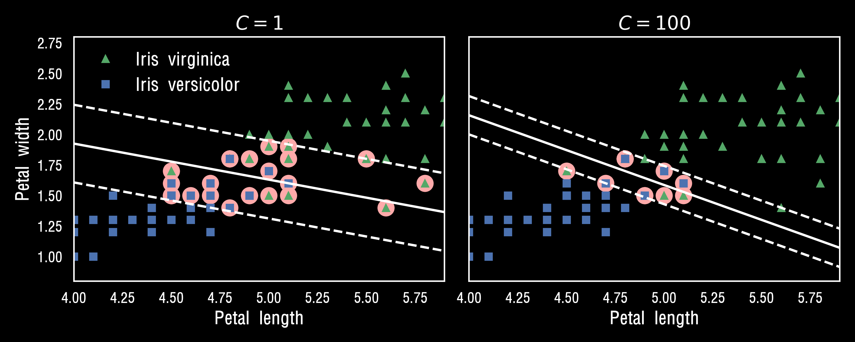
□ 비선형 SVM 분류
선형 SVM 분류기가 효율적이고 많은 경우에 아주 잘 작동하지만, 선형적으로 분류할 수 없는 데이터셋이 많습니다.
SVM이 비선형 데이터셋을 다루는 한가지 방법은 다항 특성과 같은 특성을 더 추가하는 것입니다. (ex. x^2 )
이렇게 하면 선형적으로 구분되는 데이터셋이 만들어질 수 있습니다. 아래의 왼쪽 그림은 하나의 특성 X1만을 가진 데이터셋을 나타내고 선형적으로 구분이 안됩니다.
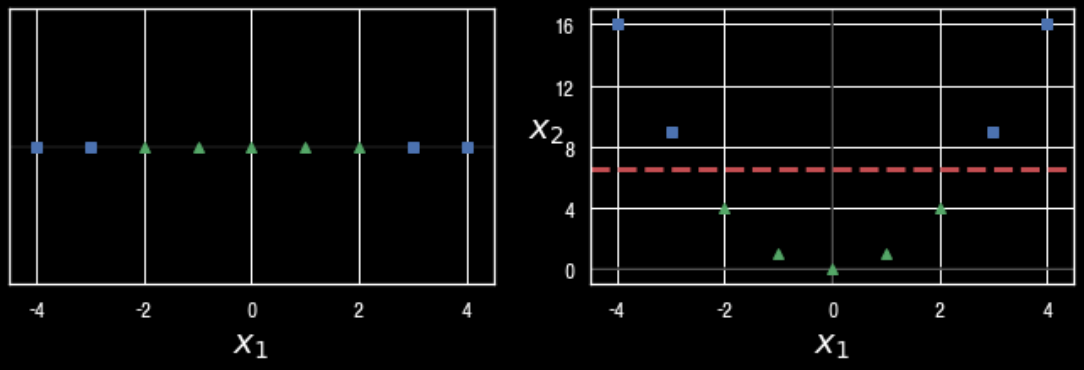
하지만 오른쪽 특성 X2=(X1)^2를 추가하여 만들어진 2차원 데이터셋은 완벽하게 선형적으로 구분할 수 있습니다.
사이킷런으로 이를 구현하려면 PolynomialFeatures변환기와 StandardScaler, LinearSVC를 연결하여 Pipeline을 만듭니다.
이를 two_moons 데이터셋에 적용해보겠습니다.
plt.style.use('seaborn-white')
plt.figure(figsize=(15,7))
from sklearn.datasets import make_moons
X, y = make_moons(n_samples=100, noise=0.15, random_state=42)

def plot_dataset(X, y, axes):
    plt.plot(X[:, 0][y==0], X[:, 1][y==0], "r^")
    plt.plot(X[:, 0][y==1], X[:, 1][y==1], "bv")
    plt.axis(axes)
    plt.grid(True, which='both')
    plt.xlabel(r"$x_1$", fontsize=20)
    plt.ylabel(r"$x_2$", fontsize=20, rotation=0)

plot_dataset(X, y, [-1.5, 2.5, -1, 1.5])
plt.show()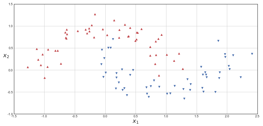
from sklearn.pipeline import Pipeline
from sklearn.preprocessing import PolynomialFeatures

polynomial_svm_clf = Pipeline([
        ("poly_features", PolynomialFeatures(degree=3)),
        ("scaler", StandardScaler()),
        ("svm_clf", LinearSVC(C=10, loss="hinge", random_state=42))
    ])

polynomial_svm_clf.fit(X, y)

>>> Pipeline(steps=[('poly_features', PolynomialFeatures(degree=3)),
                ('scaler', StandardScaler()),
                ('svm_clf', LinearSVC(C=10, loss='hinge', random_state=42))])
plt.figure(figsize=(15,7))
plt.style.use('seaborn-white')
def plot_predictions(clf, axes):
x0s = np.linspace(axes[0], axes[1], 100)
x1s = np.linspace(axes[2], axes[3], 100)
x0, x1 = np.meshgrid(x0s, x1s)
X = np.c_[x0.ravel(), x1.ravel()]
y_pred = clf.predict(X).reshape(x0.shape)
y_decision = clf.decision_function(X).reshape(x0.shape)
plt.contourf(x0, x1, y_pred, cmap=plt.cm.get_cmap('RdYlBu', 5), alpha=0.3)
plt.contourf(x0, x1, y_decision, cmap=plt.cm.get_cmap('RdYlBu', 5), alpha=0.1)
plot_predictions(polynomial_svm_clf, [-1.5, 2.5, -1, 1.5])
plot_dataset(X, y, [-1.5, 2.5, -1, 1.5])
plt.show()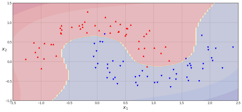
□ 다항식 커널 ( kernel="poly" )
다항식 특성을 추가하는 것은 간단하고 SVM뿐만 아니라 모든 머신러닝 알고리즘에서 잘 작동합니다.
하지만 낮은 차수의 다항식은 매우 복잡한 데이터셋을 잘 표현하지 못하고 높은 차수의 다항식은 많은 특성을 추가하므로 모델을 느리게 만듭니다.
다행히도 SVM을 사용할 땐 "커널 트릭(kernel trick)"이라는 거의 기적에 가까운 수학적 기교를 적용할 수 있습니다.
PolynomialFeature처럼 특성을 추가하지 않으면서 다항식 특성(PolynomialFeature)을 많이 추가한 것과 같은 결과를 얻을 수 있습니다.
사실 어떤 특성도 추가하지 않기때문에 엄청난 수의 특성조합이 생기지 않습니다.
from sklearn.svm import SVC

# 3차 다항식
poly_kernel_svm_clf = Pipeline([
        ("scaler", StandardScaler()),
        ("svm_clf", SVC(kernel="poly", degree=3, coef0=1, C=5))
    ])
poly_kernel_svm_clf.fit(X, y)
>>> Pipeline(steps=[('scaler', StandardScaler()),
                ('svm_clf', SVC(C=5, coef0=1, kernel='poly'))])
# 10차 다항식
poly10_kernel_svm_clf = Pipeline([
        ("scaler", StandardScaler()),
        ("svm_clf", SVC(kernel="poly", degree=10, coef0=1, C=5))
    ])
poly10_kernel_svm_clf.fit(X, y)
>>> Pipeline(steps=[('scaler', StandardScaler()),
                ('svm_clf', SVC(C=5, coef0=1, degree=10, kernel='poly'))])
이 코드는 3차 다항식 커널을 사용해 SVM 분류기를 훈련시킵니다. 결과는 아래의 시각화로 나타나있습니다.
오른쪽 그래프는 10차 다항식 커널을 사용한 또 다른 SVM분류기이고 모델이 과적합이라면 다항식의 차수를 줄여야하고 반대로 과소적합이라면 차수를 늘려야합니다
fig, axes = plt.subplots(ncols=2, figsize=(10.5, 4), sharey=True)

plt.sca(axes[0])
plot_predictions(poly_kernel_svm_clf, [-1.5, 2.45, -1, 1.5])
plot_dataset(X, y, [-1.5, 2.4, -1, 1.5])
plt.title(r"$d=3, gamma=1, C=5$", fontsize=18)

plt.sca(axes[1])
plot_predictions(poly10_kernel_svm_clf, [-1.5, 2.45, -1, 1.5])
plot_dataset(X, y, [-1.5, 2.4, -1, 1.5])
plt.title(r"$d=10, gamma=1, C=5$", fontsize=18)
plt.ylabel("")

save_fig("moons_kernelized_polynomial_svc_plot")
plt.show()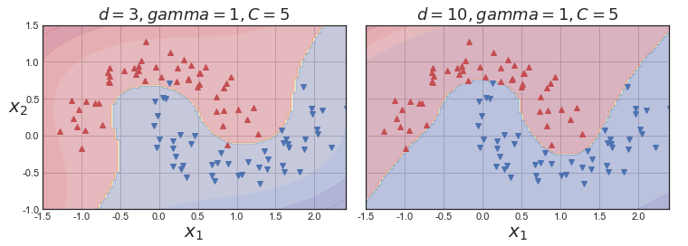
□가우시안 RBF 커널
다항 특성 방식과 마친가지로 유사도 특성방식도 머신러닝 알고리즘에 유용하게 사용될 수 있습니다.
추가 특성을 모두 계산하려면 연산비용이 많이 드는데 특히 훈련세트가 클 경우 더 그렇습니다.
여기에서 커널트릭이 한번 더 SVM의 마법(?)을 만듭니다. 유사도 특성을 많이 추가하는 것과 같은 비슷한 결과를 얻을 수 있습니다.
rbf_kernel_svm_clf = Pipeline([
        ("scaler", StandardScaler()),
        ("svm_clf", SVC(kernel="rbf", gamma=5, C=0.001))
    ])
rbf_kernel_svm_clf.fit(X, y)

>>> Pipeline(steps=[('scaler', StandardScaler()),
                ('svm_clf', SVC(C=0.001, gamma=5))])
from sklearn.svm import SVC
gamma1, gamma2 = 0.1, 5
C1, C2 = 0.001, 1000
hyperparams = (gamma1, C1), (gamma1, C2), (gamma2, C1), (gamma2, C2)
svm_clfs = []
for gamma, C in hyperparams:
rbf_kernel_svm_clf = Pipeline([
("scaler", StandardScaler()),
("svm_clf", SVC(kernel="rbf", gamma=gamma, C=C))
])
rbf_kernel_svm_clf.fit(X, y)
svm_clfs.append(rbf_kernel_svm_clf)
fig, axes = plt.subplots(nrows=2, ncols=2, figsize=(10.5, 7), sharex=True, sharey=True)
for i, svm_clf in enumerate(svm_clfs):
plt.sca(axes[i // 2, i % 2])
plot_predictions(svm_clf, [-1.5, 2.45, -1, 1.5])
plot_dataset(X, y, [-1.5, 2.45, -1, 1.5])
gamma, C = hyperparams[i]
plt.title(r"$\gamma = {}, C = {}$".format(gamma, C), fontsize=16)
if i in (0, 1):
plt.xlabel("")
if i in (1, 3):
plt.ylabel("")
plt.show()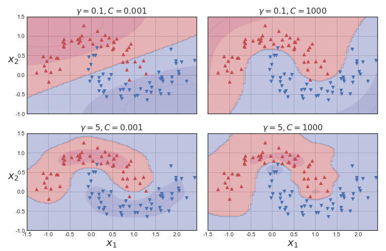
위의 시각화는 하이퍼 파라미터 gamma와 C를 바꾸어서 훈련시킬 모델입니다.
gamma를 증가시키면 종 모양 그래프가 좁아져서 각 샘플의 영향 범위가 작아집니다. 결정 경계가 조금 더 불규칙해지고 각 샘플은 따라 구불구불하게 휘어집니다.
반대로 gamma를 감소시키면 종 모양 그래프가 넓은 범위에 걸쳐 영향을 주므로 결정 경계가 더 부드러워집니다.
결국 하이퍼 파라미터 "gamma"가 규제의 역할을 합니다. 모델이 과대적합일 경우엔 감소시켜야하고, 과소적합일 경우엔 증가시켜야합니다. (하이퍼 파라미터 C와 비슷합니다.)
아래의 코드는 LinearSVM, PolynomialFeature를 적용한 SVM, Poly kernel SVM, RBF kernel SVM을 종합한 그림입니다.
linear_svm_clf = Pipeline([
        ("scaler", StandardScaler()),
        ("svm_clf", LinearSVC())
    ])
linear_svm_clf.fit(X, y)

polynomial_svm_clf = Pipeline([
        ("poly_features", PolynomialFeatures(degree=3)),
        ("scaler", StandardScaler()),
        ("svm_clf", LinearSVC(C=10, loss="hinge", random_state=42))
    ])

polynomial_svm_clf.fit(X, y)

poly_kernel_svm_clf = Pipeline([
        ("scaler", StandardScaler()),
        ("svm_clf", SVC(kernel="poly", degree=3, coef0=1, C=5))
    ])
poly_kernel_svm_clf.fit(X, y)

rbf_kernel_svm_clf = Pipeline([
        ("scaler", StandardScaler()),
        ("svm_clf", SVC(kernel="rbf", C=10))
    ])
rbf_kernel_svm_clf.fit(X, y)
fig, axes = plt.subplots(2,2, figsize=(20, 10), sharey=True)

plt.sca(axes[0,0])
plot_predictions(linear_svm_clf, [-1.5, 2.45, -1, 1.5])
plot_dataset(X, y, [-1.5, 2.4, -1, 1.5])
plt.title("Linear SVM", fontsize=18)

plt.sca(axes[0,1])
plot_predictions(polynomial_svm_clf, [-1.5, 2.45, -1, 1.5])
plot_dataset(X, y, [-1.5, 2.4, -1, 1.5])
plt.title("PolynomialFeature SVM", fontsize=18)

plt.sca(axes[1,0])
plot_predictions(poly_kernel_svm_clf, [-1.5, 2.45, -1, 1.5])
plot_dataset(X, y, [-1.5, 2.4, -1, 1.5])
plt.title("Poly kernel SVM", fontsize=18)

plt.sca(axes[1,1])
plot_predictions(rbf_kernel_svm_clf, [-1.5, 2.45, -1, 1.5])
plot_dataset(X, y, [-1.5, 2.4, -1, 1.5])
plt.title("RBF kernel SVM", fontsize=18)

plt.show()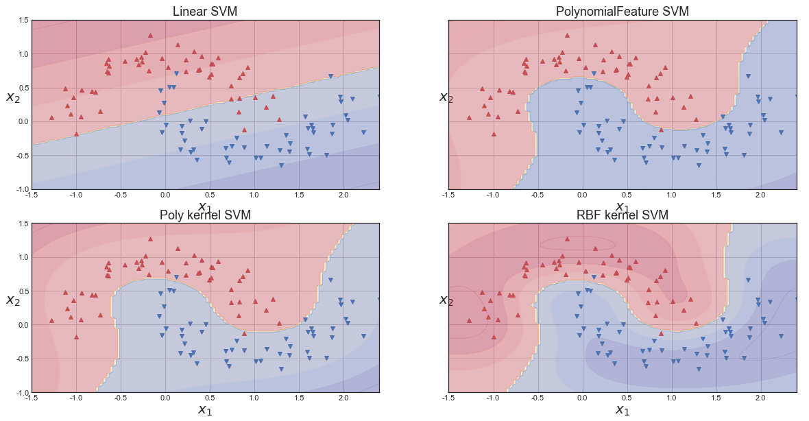
보시는 바와 같이 보편적으로 RBF kernel을 쓰는 이유는 가장 우수한 성능을 나타내기때문에 쓰는 것이라 보입니다.
이번엔 SVM은 어떠한 결정 경계를 띄는 지 보고 글을 마치도록 하겠습니다
# 데이터 생성
from sklearn.datasets import make_circles
from sklearn.datasets import make_moons
X_c, y_c = make_circles(n_samples=100, factor=0.3, noise=0.25, random_state=0)
X_m,y_m = make_moons(n_samples=100, noise=0.25, random_state=0)

from sklearn.datasets import make_classification
X_clf, y_clf = make_classification(
    n_features=2, n_redundant=0, n_informative=2, random_state=1, n_clusters_per_class=1
)
rng = np.random.RandomState(2)
X_clf += 2 * rng.uniform(size=X_clf.shape)
fig, axes = plt.subplots(1,3, figsize=(20,7))
mglearn.discrete_scatter(X_c[:,0],X_c[:,1], y_c , ax=axes[0])
mglearn.discrete_scatter(X_m[:,0],X_m[:,1], y_m , ax=axes[1])
mglearn.discrete_scatter(X_clf[:,0],X_clf[:,1],y_clf, ax=axes[2])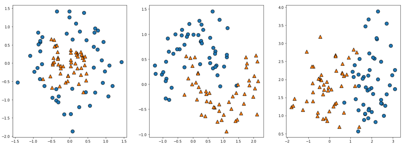
fig,axes = plt.subplots(1,4,figsize=(30,7))
for kernel, ax in zip(['rbf','poly','linear','sigmoid','precomputed'], axes):
    svm_c = SVC(kernel = kernel).fit(X_c, y_c)
    mglearn.plots.plot_2d_separator(svm_c ,X_c ,fill=True , eps=0.3, ax=ax, alpha=0.5)
    mglearn.discrete_scatter(X_c[:,0],X_c[:,1],y_c,ax=ax)
    ax.set_title("kernel = {}".format(kernel), bbox=dict(facecolor='violet'), fontdict={'size':15})
    ax.set_xlabel("feature 0")
    ax.set_ylabel("feature 1")
axes[0].legend(loc=3)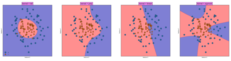
fig,axes = plt.subplots(1,4,figsize=(30,7))
for kernel, ax in zip(['rbf','poly','linear','sigmoid','precomputed'], axes):
    svm_m = SVC(kernel = kernel).fit(X_m, y_m)
    mglearn.plots.plot_2d_separator(svm_m ,X_m ,fill=True , eps=0.5, ax=ax, alpha=0.6)
    mglearn.discrete_scatter(X_m[:,0],X_m[:,1],y_m, alpha=0.6,ax=ax)
    ax.set_title("kernel = {}".format(kernel), bbox=dict(facecolor='violet'), fontdict={'size':15})
    ax.set_xlabel("feature 0")
    ax.set_ylabel("feature 1")
axes[0].legend(loc=3)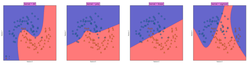
fig,axes = plt.subplots(1,4,figsize=(30,7))
for kernel, ax in zip(['rbf','poly','linear','sigmoid','precomputed'], axes):
    svm_clf = SVC(kernel = kernel).fit(X_clf, y_clf)
    mglearn.plots.plot_2d_separator(svm_clf ,X_clf ,fill=True , eps=0.5, ax=ax, alpha=0.4)
    mglearn.discrete_scatter(X_clf[:,0],X_clf[:,1],y_clf,ax=ax)
    ax.set_title("kernel = {}".format(kernel), bbox=dict(facecolor='violet'), fontdict={'size':15})
    ax.set_xlabel("feature 0")
    ax.set_ylabel("feature 1")
axes[0].legend(loc=3)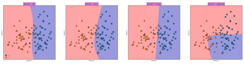
이상으로 [Python/ML] SVM (Support Vector Machine)를 마치도록 하겠습니다.
질문 혹은 궁금한 사항은 댓글로 남겨주시고 오늘도 긴 글 읽어주셔서 대단히 감사드립니다.
참고) scikit-learn SVC
https://scikit-learn.org/stable/modules/classes.html?highlight=svm#module-sklearn.svm
API Reference
This is the class and function reference of scikit-learn. Please refer to the full user guide for further details, as the class and function raw specifications may not be enough to give full guidel...
scikit-learn.org
https://book.naver.com/bookdb/book_detail.naver?bid=22059668
파이썬 라이브러리를 활용한 머신러닝 : 네이버 도서
네이버 도서 상세정보를 제공합니다.
search.shopping.naver.com
'Data Park > Python' 카테고리의 다른 글
| [Python/ML] K-MEANS Clustering (0) | 2023.01.27 |
|---|---|
| [Python/ML] K-NN (K-Nearest Neighbors) (0) | 2023.01.10 |
| [Python/ML] Ada Boosting, Gradient Boosting (0) | 2022.12.11 |
| [Python/ML] Random Forest (랜덤 포레스트) (1) | 2022.12.10 |
| [Python/ML] Decision Tree (의사결정나무) (0) | 2022.12.10 |


