[Python/NLP] 네이버 영화 리뷰 감성 분석

분석 환경 : 코랩

※ 환경 설정

□ 폰트 설정 - 나눔고딕체

## colab 환경에서 한글 폰트 설정
!sudo apt-get install -y fonts-nanum
!sudo fc-cache -fv
!rm ~/.cache/matplotlib -rf
import matplotlib.pyplot as plt
plt.rc('font', family='NanumBarunGothic') 
plt.title('안녕')

□ KoNLPy(코앤엘파이) 설치

## colab 환경에서 konlpy 설정 

%%bash
apt-get update
apt-get install g++ openjdk-8-jdk python-dev python3-dev
pip3 install JPype1
pip3 install konlpy

%env JAVA_HOME "/usr/lib/jvm/java-8-openjdk-amd64"

□ 데이터 불러오기

import pandas as pd
from sklearn.metrics import accuracy_score, classification_report,confusion_matrix, plot_confusion_matrix
import matplotlib.pyplot as plt
import seaborn as sns
import plotly.express as px
import urllib.request
urllib.request.urlretrieve("https://raw.githubusercontent.com/e9t/nsmc/master/ratings_train.txt", filename="ratings_train.txt")
urllib.request.urlretrieve("https://raw.githubusercontent.com/e9t/nsmc/master/ratings_test.txt", filename="ratings_test.txt")
train_df = pd.read_table('ratings_train.txt')
test_df = pd.read_table('ratings_test.txt')
train_df

test_df

□ 전처리 1. traing, test data 병합

• 초기의 방법은 15만건/5만건으로 수행해보았는데, 더 이상 정확도를 올릴 방법을 고안하지 못하였다
• 원래는 train_set=150000건 // test_set=50000건 (75%:25%)이어서 학습할 데이터가 적어 정확도가 낮은 것일 수도 있겠다란 생각에서 착안된 방법
• 따라서 75:25뿐만 아니라 90:10, 80:20, 60:40 등 다양한 샘플링 방법을 사용한다.

raw_df = train_df.append(test_df, ignore_index = True)
raw_df

□ 전처리 2. 결측치 삭제

# 결측치 확인
raw_df[raw_df['document'].isna()]

# 결측치 제거
raw_df = raw_df[raw_df['document'].notnull()]
raw_df

□ 전처리 3. 정규화

# 정규화
import re 
raw_df['document'] = raw_df['document'].apply(lambda x : re.sub(r'[^ ㄱ-ㅣ가-힣]+', " ", str(x)))
raw_df

□ 전처리 4. X, y 할당

# input, output 데이터를 X, y에 각각 분할
X = raw_df.drop("label", axis = 1)
y = raw_df['label']
X['document'], y

□ 전처리 4-1. 단어길이 빈도 생성 및 EDA 시각화

# 단어 길이 빈도
raw_word_counts = raw_df['document'].apply(lambda x:len(x.split(' ')))

import plotly.figure_factory as ff
fig = px.histogram(raw_word_counts, template="plotly_dark", color=raw_word_counts,  
                   title= "문장 길이 시각화")
fig.update_layout(height = 600, width = 1000, hovermode = 'closest')
fig.show()

# 리뷰의 단어개수
plt.figure(figsize=(15,10))
plt.hist(raw_word_counts , bins=50, facecolor='r',label='train')
plt.title('Log-Histogram of word count in review',fontsize=15)
plt.yscale('log',nonposy='clip')
plt.legend()
plt.xlabel('Number of words',fontsize=15)
plt.ylabel('Number of reviews', fontsize=15)

□ 워드 클라우드

from wordcloud import WordCloud, STOPWORDS
stopwords = ['영화는','아','다','그냥','진짜','너무','의','정말','영화','가','이','은','들','는','좀','잘','걍','과','도','를','으로','자','에','와','한','하다']
%matplotlib inline

wordcloud1 = WordCloud(font_path='NanumBarunGothic.ttf',
                      stopwords = stopwords, 
                      colormap='Set3', 
                      background_color = 'black', 
                      width = 800, height = 600).generate(' '.join(raw_df['document']))

plt.figure(figsize = (15, 10))
plt.imshow(wordcloud1)
plt.axis("off")
plt.show()

□ 전처리 5. train, test set 분할

from sklearn.model_selection import train_test_split
# train, test 9:1로 분할 비율이 가장 성능이 좋았음
X_train, X_test, y_train, y_test = train_test_split(X, y, 
                                                    test_size=0.1, 
                                                    random_state=None, 
                                                    shuffle=True, 
                                                    stratify=y)

# train set 확인
X_train, y_train

# test set 확인
X_test, y_test

□ 전처리 6. Vectorizer (문자를 숫자로 바꿔준다)

from konlpy.tag import Okt
okt = Okt()
def okt_tokenizer(text):
    tokens = okt.morphs(text)
    return tokens
    
import time
start = time.time()
#---------------------------------------------
from sklearn.feature_extraction.text import TfidfVectorizer

tfidf = TfidfVectorizer(tokenizer=okt_tokenizer, ngram_range=(1,1), min_df=3 , max_df=0.9)
tfidf.fit(X_train['document'])
train_tfidf = tfidf.transform(X_train['document'])
test_tfidf = tfidf.transform(X_test['document'])
#----------------9:1로 나눴을때 18분 걸림-------
end = time.time() 
print('토큰화 수행 시간 :') 
print(end - start)

train_tfidf

□ 전처리 6-1. 모델링하기전 마지막 확인

# 0,1의 비율을 동일하게 맞춤 => 업샘플링, 다운샘플링이 필요없음
y_train.value_counts()

>>> 
1    89996
0    89996
Name: label, dtype: int64


y_test.value_counts()

>>>
1    10000
0    10000
Name: label, dtype: int64

□ 모델링 1. 로지스틱 회귀 분류기

from sklearn.linear_model import LogisticRegression
from sklearn.metrics import accuracy_score, classification_report,confusion_matrix, plot_confusion_matrix
from sklearn.metrics import accuracy_score, precision_score , recall_score
### 로지스틱 회귀 ###
start = time.time()
#----------------------------------------------
lr = LogisticRegression(C=5 , random_state=0)

lr.fit( train_tfidf, y_train )
lr_pred = lr.predict( test_tfidf )
lr_acc = lr.score( test_tfidf, y_test )
#----------------------------------------------
print("로지스틱 회귀 training accuracy :", lr.score( train_tfidf , y_train )*100, "%")
print("로지스틱 회귀 testing accuracy :", lr_acc * 100, "%")
print("--------------------------------------------------------------------------")
print(classification_report( y_test, lr_pred ))
print("--------------------------------------------------------------------------")
print(confusion_matrix( y_test, lr_pred ))
print("--------------------------------------------------------------------------")
#----------------------------------------------
end = time.time() 
print('로지스틱 회귀 수행시간 :') 
print(end - start)

plt.figure(figsize=(20, 20))
plot_confusion_matrix(lr , test_tfidf , y_test , cmap='Blues')
plt.title("<< Logistic Regression_박성호 >>")

로지스틱 회귀 training accuracy : 94.45419796435397 %
로지스틱 회귀 testing accuracy : 86.375 %
--------------------------------------------------------------------------
              precision    recall  f1-score   support

           0       0.86      0.87      0.86     10000
           1       0.87      0.86      0.86     10000

    accuracy                           0.86     20000
   macro avg       0.86      0.86      0.86     20000
weighted avg       0.86      0.86      0.86     20000

--------------------------------------------------------------------------
[[8700 1300]
 [1425 8575]]
--------------------------------------------------------------------------
로지스틱 회귀 수행시간 :
14.776463508605957

# LogisticRegression Cross Validation
import numpy as np
from sklearn.model_selection import cross_val_score, cross_validate
scores_lr = cross_val_score(lr, train_tfidf, y_train , cv=5)
print("로지스틱 회귀 교차 검증 정확도: {}".format(scores_lr))
print("로지스틱 회귀 교차 검증 정확도:{} +/- {}".format(np.mean(scores_lr),np.std(scores_lr))) #정확도평균+-오차

>>> 로지스틱 회귀 교차 검증 정확도: [0.8587183  0.86002389 0.86143675 0.86035335 0.85776988]
>>> 로지스틱 회귀 교차 검증 정확도:0.8596604325674356 +/- 0.0012829148517790696

그 당시 과제에서 정확도를 올리는 것이 가장 큰 목적이었고 무슨 방법이던 다 써서 어떻게든 정확도를 올려야했다.

from sklearn.model_selection import GridSearchCV   #효과적인 하이퍼 파라미터 세팅을 찾아줌
from sklearn.linear_model import LogisticRegression
import numpy as np

lr = LogisticRegression( random_state = 0 )

params = {'C' : [3, 3.5, 4, 4.5, 5, 6],
          'max_iter' : [10, 50, 100, 1000],
          "penalty":["l1","l2"]
          }
lr_grid_cv = GridSearchCV(lr, param_grid=params, cv=3, scoring='accuracy', verbose=1)


>>> GridSearchCV(cv=3, estimator=LogisticRegression(random_state=0),
                 param_grid={'C': [3, 3.5, 4, 4.5, 5, 6],
                             'max_iter': [10, 50, 100, 1000],
                             'penalty': ['l1', 'l2']},
                 scoring='accuracy', verbose=1)

import time
start = time.time()
#----------------------------------------------
lr_grid_cv.fit(test_tfidf, y_test)
print("로지스틱 최적 점수 : {}".format(lr_grid_cv.best_score_))
print("로지스틱 최적 파라미터 : {}".format(lr_grid_cv.best_params_))
print(lr_grid_cv.best_estimator_)
#----------------------------------------------
end = time.time() 
print("--------------------------------------------------------------------------")
print('Execution time is:') 
print(end - start)


>>> 로지스틱 최적 점수 : 0.8149501390817049
>>> 로지스틱 최적 파라미터 : {'C': 4.5, 'max_iter': 100, 'penalty': 'l2'}
>>> LogisticRegression(C=4.5, random_state=0)
>>> --------------------------------------------------------------------------
>>> Execution time is:
>>> 124.36003136634827

또 그리드 서치를 돌려보면서 느낀 것은 C=4.5가 가장 성능이 좋대서 써봤는데 아니더라 큰 차이 없고 오히려 낮아졌다,, 이런 대용량의 거대 corpus에서 그리드 서치는 좋은 성능으로 높이기엔 한계가 있는 것으로 보인다.

□ 모델링 2. 나이브 베이즈 분류기

from sklearn.naive_bayes import ComplementNB
import matplotlib.pyplot as plt
start = time.time()
nb_clf = ComplementNB(alpha = 0.5)
nb_clf.fit(train_tfidf, y_train)
nb_pred = nb_clf.predict( test_tfidf )
nb_acc = nb_clf.score( test_tfidf , y_test )
print("Naive Bayes training accuracy :", nb_clf.score( train_tfidf , y_train )*100, "%")
print("Naive Bayes testing accuracy :", nb_acc * 100, "%")
print("--------------------------------------------------------------------------")
print(classification_report(y_test, nb_pred))
print("--------------------------------------------------------------------------")
print(confusion_matrix(y_test, nb_pred))
print("--------------------------------------------------------------------------")
plot_confusion_matrix(nb_clf, test_tfidf , y_test, cmap='Greys')
plt.title("Complement Naive Bayes, Acc=86.165")
end = time.time() 
print("--------------------------------------------------------------------------")
print('Execution time is:') 
print(end - start)

Naive Bayes training accuracy : 90.51124494421975 %
Naive Bayes testing accuracy : 86.46000000000001 %
--------------------------------------------------------------------------
              precision    recall  f1-score   support

           0       0.86      0.88      0.87     10000
           1       0.87      0.85      0.86     10000

    accuracy                           0.86     20000
   macro avg       0.86      0.86      0.86     20000
weighted avg       0.86      0.86      0.86     20000

--------------------------------------------------------------------------
[[8771 1229]
 [1479 8521]]

사실 나이브 베이즈를 안쓸려했지만 예상외로 성능도 좋고 수행시간도 굉장히 빨랐다.

내가 앙상블 모델에만 너무 집중을 해서 로지스틱과 나이브 베이즈같은 통계의 기본이 되는 모델들은 안중 밖이었다.

하지만 이 프로젝트를 진행하면서 반성했다.^^

params = {'alpha': [0.3, 0.45, 0.5, 0.55, 0.8]
         }
nb_clf = ComplementNB()
nb_grid_cv = GridSearchCV(nb_clf, param_grid=params, cv=3, scoring='accuracy', verbose=1)
import time
start = time.time()
#----------------------------------------------
nb_grid_cv.fit(train_tfidf, y_train)
print("나이브 베이즈 최적 점수 : {}".format(nb_grid_cv.best_score_))
print("나이브 베이즈 최적 파라미터 : {}".format(nb_grid_cv.best_params_))
print(nb_grid_cv.best_estimator_)
#----------------------------------------------
end = time.time() 
print("--------------------------------------------------------------------------")
print('Execution time is:') 
print(end - start)

# 결과
Fitting 3 folds for each of 5 candidates, totalling 15 fits
나이브 베이즈 최적 점수 : 0.8584937173974788
나이브 베이즈 최적 파라미터 : {'alpha': 0.45}
ComplementNB(alpha=0.45)
--------------------------------------------------------------------------
Execution time is:
1.2268147468566895

□ 모델링 결과

엄층 다양한 알고리즘을 써봤지만 내가 확신했고 중간고사부터 내 인생을 갈아넣은 앙상블 모델은 교수님의 간단한 로지스틱에 처참히 전멸해버렸다,,,

# 0806
import pandas as pd
import seaborn as sns
import matplotlib.pyplot as plt
import numpy as np
models_acc = {'Logistic Regression':86.375 , 
              'Naive Bayse':86.460 , 
              'SVM':85.937, 
              'LighGBM':84.74 , 
              'Random Forest': 81.97 , 
              'K-NN':60.175 , 
              }

models_acc_df = pd.DataFrame(pd.Series(models_acc))
models_acc_df.columns = ['정확도']
models_acc_df['모델'] = ['Logistic Regression', 'Naive Bayse', 'SVM', 
                          'LighGBM', 'Random Forest', 'K-NN']
models_acc_df.set_index(pd.Index([1, 2 , 3 , 4 , 5 , 6]))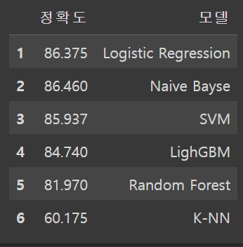

import plotly.express as px
fig = px.bar(models_acc_df, x='정확도', y='모델' ,color='모델', range_x=(50,90), template="plotly_dark", text_auto='.4s',
            title="<<심화기계학습 최종 모델평가>> by 박성호" )
fig.update_traces(textfont_size=15, textangle=0, textposition="inside", cliponaxis=False)
fig.update_yaxes(categoryorder="total ascending")
fig.update_layout(height = 600, width = 1000, hovermode = 'closest')
fig.update_layout(coloraxis = {'colorscale':'Bluered_r'})

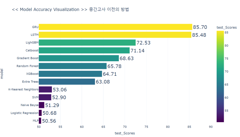
느낀점)

tf-idf를 배우기 전 CountVectorizer()로 딥러닝 LSTM, GRU 모델까지 돌렸는데 85%의 정확도가 나왔지만, 딥러닝을 설명하기 위해서는 추가적인 공부가 필요했다.

tf-idf를 배운 후엔 로지스틱을 돌려보니 딥러닝 모델에 준하는 성능이 뽑혔다. 그야말로 감동실화였다.

이 다음에 tf-idf하고 딥러닝 모델로 수행해보면 얼마나 높아질까. 궁금하다

# 새로운 텍스트를 직접 입력해 감성 예측 수행해봅시다!
st = input("감성을 분석할 문장을 입력하세요: ")

>>> 1. 감성을 분석할 문장을 입력하세요: 박성호가 찢었다,,, 개꿀잼이네
>>> 2. 감성을 분석할 문장을 입력하세요: 와,,, 이런 것도 상품이라고 차라리 내가 만드는 게 나을 뻔ㅋㅋ

st = re.compile(r'[ㄱ-ㅣ가-힣]+').findall(st)
print(st)

st = [" ".join(st)]
print(st)

>>> ['박성호가', '찢었다', '개꿀잼이네']
>>> ['박성호가 찢었다 개꿀잼이네']

>>> ['와', '이런', '것도', '상품이라고', '차라리', '내가', '만드는', '게', '나을', '뻔ㅋㅋ']
>>> ['와 이런 것도 상품이라고 차라리 내가 만드는 게 나을 뻔ㅋㅋ']​

# 입력 텍스트의 벡터화
st_tfidf = tfidf.transform(st)

# 감성 분석 모델에 적용하여 예측
st_predict = nb_clf.predict(st_tfidf)
# 예측값 출력
if(st_predict ==0):
    print(st, "->> 부정 감성")
else:
    print(st, "->> 긍정 감성")
    
    
>>> 1. ['박성호가 찢었다 개꿀잼이네'] ->> 긍정 감성
>>> 2. ['와 이런 것도 상품이라고 차라리 내가 만드는 게 나을 뻔ㅋㅋ'] ->> 부정 감성​

참고)

10-06 네이버 영화 리뷰 감성 분류하기(Naver Movie Review Sentiment Analysis)